I. Generation of Simulation Data:
To clearly present the analysis results, post-infection clinical symptoms of the virus are simulated using the common case-control pattern, simulating both severe and mild patients. Considering that some clinical phenotypic data (such as age) are highly correlated with post-infection symptoms, we set up 2 strongly correlated features. Additionally, we established 20 features with varying degrees of linear correlation, 3 non-linearly correlated features, and 20 noise-unrelated features, totaling 45 feature data. Infection patient samples were divided into three categories, each generated with different random seed numbers: including 500 training samples, 300 validation samples, and 300 independent test samples. Considering the potential for partial data missing in reality, a small amount of missing data (marked as NA) was introduced into the simulation data. This missing data was addressed through imputation methods during analysis.
II. Artificial Intelligence Analysis Process and Results:
Two methods were used for analysis.
1). Four common machine learning methods were chosen: Random Forest (rf), Support Vector Machine (SVM), K Nearest Neighbors (KNN), and glmnet. These were integrated using the greedy ensemble method. Features were extracted from the training samples, parameters optimized, the best features and models selected through validation samples, and final predictions obtained through independent sample tests.

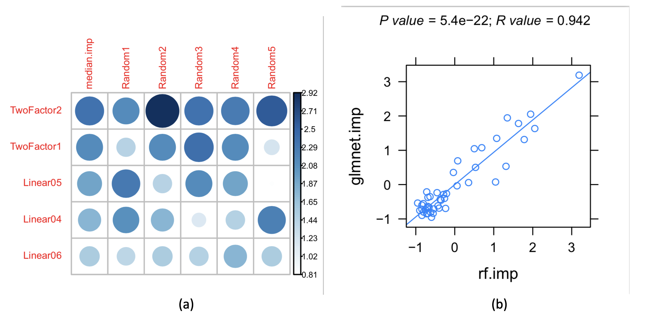
Figure 1: (a) Feature importance ranking based on the glmnet algorithm, with two types of strongly correlated features and linearly correlated features ranked at the front; (b) The importance rankings obtained by the glmnet and random forest (rf) algorithms are highly correlated, revealing the stability of the results.
a) Features were sorted by correlation, as shown in Figure 1, revealing that two strongly correlated features and linearly correlated features were ranked upfront. The importance ranking of features based on glmnet algorithm and the high correlation between glmnet and rf algorithms in importance ranking, indicating the stability of the results.
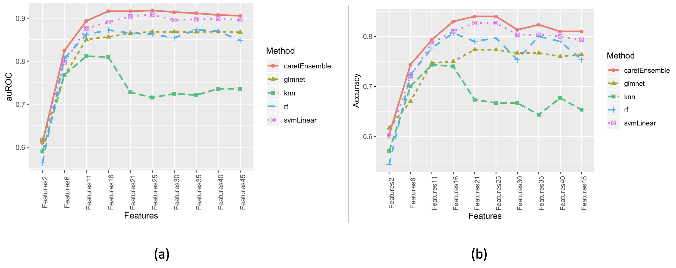
b) Features were sorted by importance and grouped. Four different algorithms were used for modeling, and finally integrated using the greedy ensemble method. The prediction results for the validation group samples are shown in Figure 2. It can be concluded from Figure 2 that the ensemble algorithm, after integration of four algorithms, achieved the optimal model with a combination of 25 features. This conclusion aligns well with our simulated feature generation: 2 strongly correlated, 20 linearly correlated, and 3 non-linearly correlated.

Figure 2: Performance of Different Feature Combinations in the Validation Group Samples: (a) Area Under the Receiver Operating Characteristic Curve (auROC); (b) Accuracy.
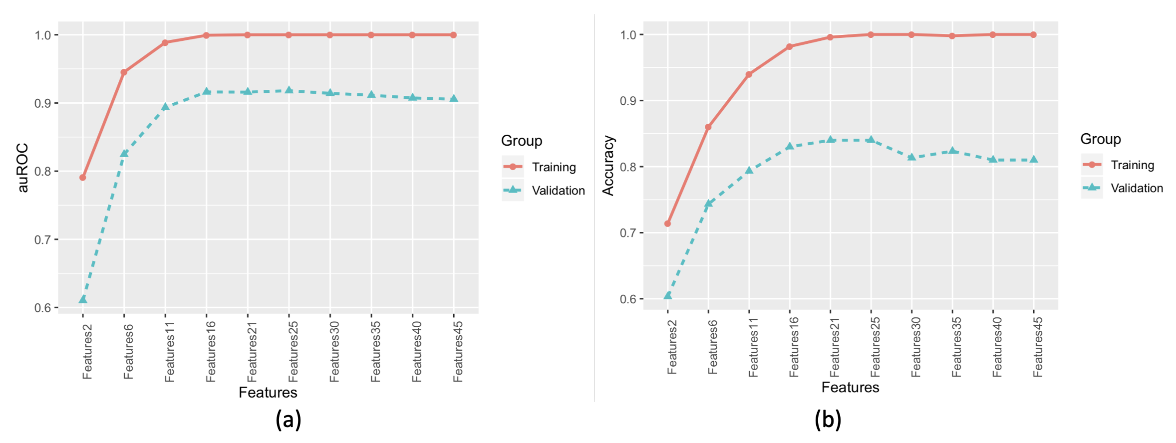
c) By combining the prediction data of the training group and the validation group ensemble models, it can be observed that the phenomenon of under-fitting and over-fitting in the training group was best resolved with 25 features (Figure 3). Under-fitting occurred before 16 features, and over-fitting after 25 features.

Figure 3: Prediction Results of the Ensemble Model for the Training and Validation Groups: (a) Area Under the Receiver Operating Characteristic Curve (auROC); (b) Accuracy.
d) The ensemble model with 25 features was used to validate 300 independent samples, with prediction results and the auROC curve shown in Figure 4. The AUC of the prediction results was 0.957, with an overall prediction accuracy of 0.883.


2). Deep Learning Method
a) The analysis used the Keras deep learning framework, with a two-layer hidden structure model design, and a maximum of 100 analysis cycles (epochs).
b) Training and validation sample sets were merged and randomly re-divided into 70% (560 samples) for the training set, and 30% (240 samples) for the validation set, keeping the independent validation samples unchanged. Accuracy and loss data for the training and validation sets are shown in Figure 5. The accuracy peaked around 60 epochs, indicating the optimal model.
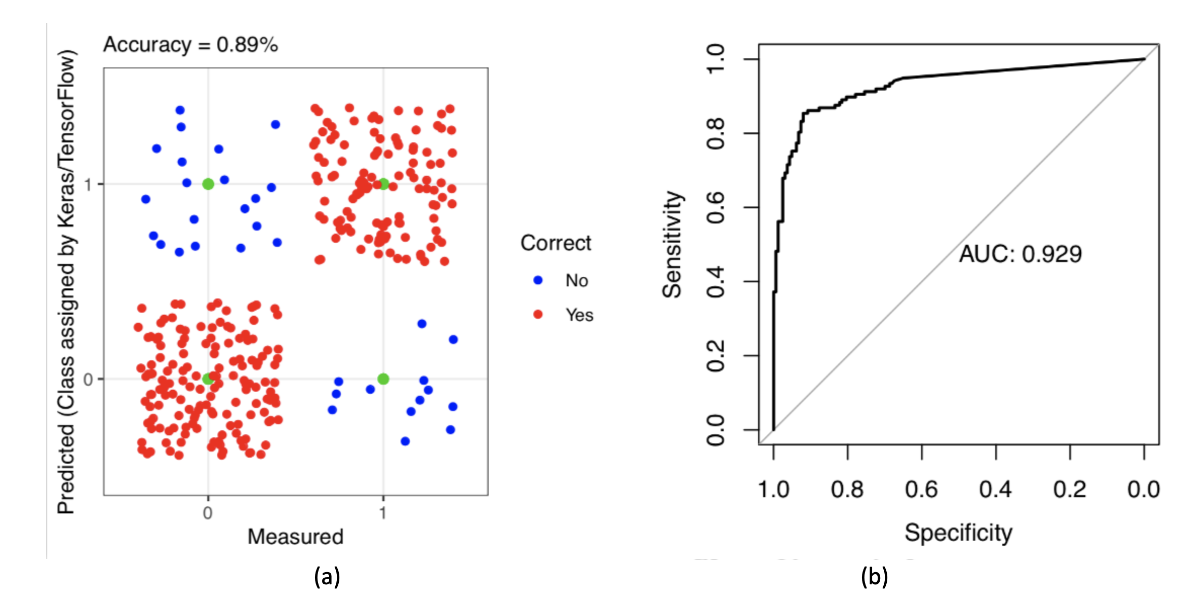
c) For 300 independent sample validations, the accuracy was 0.89, and the AUC was 0.93 (Figure 6).

Figure 6: Deep Learning Validation Results for 300 Independent Samples: (a) Density Distribution of Prediction Results; (b) Area Under the Receiver Operating Characteristic Curve (auROC).
III. Summary:
Based on actual media reports and communication with frontline doctors, we speculated the degree of correlation between post-COVID-19 infection symptoms and clinical data. We simulated 1100 samples and 45 feature data, using two analysis methods: 1) an ensemble of 4 traditional machine learning algorithms; 2) deep learning, to observe the predictive ability of AI models for post-viral infection symptoms. Further testing showed that if the training samples increased to 2000, with 300 validation samples and 300 test samples unchanged, the independent validation AUC could reach 0.97, with an accuracy rate of 0.92. The independent sample prediction results of both methods were similar, and all indicators showed good predictive performance, further proving the feasibility of predicting post-COVID-19 infection symptoms using artificial intelligence methods.
